Tech Note Demo

This notebook reproduces the figures from the mzapy tech note, and serves as a demonstration of the package’s functionality. The data file used in this demo can be found here.

To download and run this demo notebook, first download the data file from the link above, then at the top of this page click “View page source”, then right-click and save as “demo.ipynb” on your machine.

Imports

from matplotlib import pyplot as plt, rcParams
import numpy as np

from mzapy import MZA
from mzapy.isotopes import MolecularFormula, monoiso_mass, predict_m_m1_m2, ms_adduct_mz
from mzapy.peaks import find_peaks_1d_gauss, find_peaks_1d_localmax
from mzapy.calibration import MassCalibration, CCSCalibrationDTsf
from mzapy.view import (
    plot_chrom, plot_spectrum, plot_atd, add_peaks_to_plot,
    plot_mass_calibration, plot_dtsf_ccs_calibration
)

Setup

# increase the font size to make rendered plots more legible
rcParams['font.size'] = 10

# calculate some info for PC(18:0/18:1) [M+H]+ (C44H87NO8P)
pc_formula = MolecularFormula(C=44, H=87, N=1, O=8, P=1)
pc_mz = monoiso_mass(pc_formula)
pc_iso_masses, pc_iso_abun = predict_m_m1_m2(pc_formula)

# load the MZA file
mza = MZA('demo_data.mza', mza_version='old')

Extract and View XIC

# extract the chromatogram for the monoiso m/z +/- 0.02
mz_min, mz_max = pc_mz - 0.02, pc_mz + 0.02
xic_rt, xic_i = mza.collect_xic_arrays_by_mz(mz_min, mz_max)

# plot TIC and XIC, without fit
print('TIC and XIC (no fitting)')
ax = plot_chrom(*mza.collect_xic_arrays_by_mz(mza.min_mz, mza.max_mz),
                c='grey', label='TIC', figsize=(5.5, 2.5))
ax2 = ax.twinx()
for d in ['top', 'left', 'bottom']:
    ax2.spines[d].set_visible(False)
ax.legend(frameon=False, loc='upper left')
plot_chrom(xic_rt, xic_i,
           ax=ax2, figname='show', label='XIC')

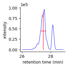
# fit XIC to get the obs. retention time, plot fitted RT for two peaks
pk_means, pk_heights, pk_widths = find_peaks_1d_gauss(xic_rt, xic_i,
                                                      0.05, 1e3, 0.05,
                                                      2, 1, True)
# only look for the most intense peak
pk_mean, pk_height, pk_width = pk_means[0], pk_heights[0], pk_widths[0]

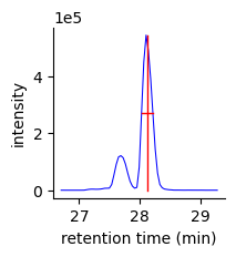
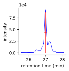
# plot the region around the fitted chromatographic peak
print('XIC with gaussian fit')
ax = plot_chrom(xic_rt, xic_i,
                rt_range=[pk_mean - 3, pk_mean + 3], figsize=(5, 2.5))

# annotate with the fitted peak
add_peaks_to_plot(ax, pk_means, pk_heights, pk_widths,
                  add_text_lbl=True, x_units='min', fontsize=8)

# show the plot and close
plt.show()
plt.close()

TIC and XIC (no fitting)

XIC with gaussian fit

Extract and View MS1 Spectra

# extract MS1 spectrum from fitted RT +/- FWHM (full m/z range)
rt_min, rt_max = pk_mean - pk_width, pk_mean + pk_width
ms1_mz, ms1_i = mza.collect_ms1_arrays_by_rt(rt_min, rt_max)

# fit the region right around the monoisotopic mass to get the peak height of the monoisotopic peak
ms1_pk_height = find_peaks_1d_localmax(
    *mza.collect_ms1_arrays_by_rt(rt_min, rt_max,
                                  mz_bounds=(pc_mz - 0.5, pc_mz + 0.5)),
    0.05, 1e3, 0.01, 1, 0.2)[1][0]

# plot MS1 spectrum, full m/z range
print('MS1 spectrum (full m/z range)')
plot_spectrum(ms1_mz, ms1_i, figname='show', figsize=(5.5, 2.5))

# plot MS1 spectrum, M - 1.5 to M + 3.5
# annotate with bars corresponding to theoretical isotope distribution
print('MS1 spectrum (M - 1.5 to M + 3.5)')
ax = plot_spectrum(*mza.collect_ms1_arrays_by_rt(mza.min_rt, mza.max_rt,
                                                 mz_bounds=(pc_mz - 1.5, pc_mz + 3.5)),
                   mz_range=(pc_mz - 1.5, pc_mz + 3.5), c='grey', label='full', figsize=(5.5, 2.5))
plot_spectrum(ms1_mz, ms1_i,
              mz_range=(pc_mz - 1.5, pc_mz + 3.5), ax=ax, label='RT sel.')
ax.bar(pc_iso_masses, [_ * ms1_pk_height for _ in pc_iso_abun],
       width=0.025, color='r', zorder=2)
ax.legend(frameon=False)

# show the plot and close
plt.show()
plt.close()

MS1 spectrum (full m/z range)

MS1 spectrum (M - 1.5 to M + 3.5)

Extract and View ATD

# extract RT and m/z selected ATD
atd_dt, atd_i = mza.collect_atd_arrays_by_rt_mz(mz_min, mz_max, rt_min, rt_max)

# It takes a very long time to get the non-RT-selected ATD, so don't run this every time
# plot ATD
ax = plot_atd(*mza.collect_atd_arrays_by_rt_mz(mz_min, mz_max, mza.min_rt, mza.max_rt),
              c='grey', ls='--', label='full', figsize=(5.5, 2.5))
plot_atd(atd_dt, atd_i, label='RT sel.', ax=ax)
ax.legend(frameon=False)

# show the plot and close
print('ATD with and without RT selection')
plt.show()
plt.close()

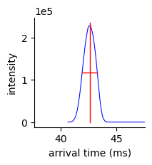
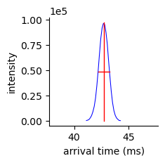
# fit ATD to get observed drift time
atd_means, atd_heights, atd_widths = find_peaks_1d_gauss(atd_dt, atd_i,
                                                         0.05, 1e3, 1,
                                                         20, 1, True)
atd_mean, atd_height, atd_width = atd_means[0], atd_heights[0], atd_widths[0]

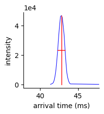
# plot the ATD with fit
ax = plot_atd(atd_dt, atd_i,
              dt_range=[atd_mean - 8, atd_mean + 8], figsize=(5.25, 2.5))

# annotate with the fitted peak
add_peaks_to_plot(ax, atd_means, atd_heights, atd_widths,
                  add_text_lbl=True, x_units='ms', fontsize=8)

# show the plot and close
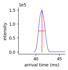
print('ATD with gaussian fit')
plt.show()
plt.close()

ATD with and without RT selection

ATD with gaussian fit

Mass Calibration

# use some TGs from this sample as mass calibrants
# lipid id, molecular formula (neutral), ionization, expected retention time
mass_calibrants = [
    ['TG(50:1)', MolecularFormula(C=53, H=100, O=6), '[M+NH4]+', 27.709],
    ['TG(52:4)', MolecularFormula(C=55, H=98, O=6), '[M+NH4]+', 24.1],
    ['TG(52:3)', MolecularFormula(C=55, H=100, O=6), '[M+NH4]+', 27.253],
    ['TG(52:1)', MolecularFormula(C=55, H=104, O=6), '[M+NH4]+', 28.165],
    ['TG(54:5)', MolecularFormula(C=57, H=100, O=6), '[M+NH4]+', 26.836],
    ['TG(54:2)', MolecularFormula(C=57, H=106, O=6), '[M+NH4]+', 28.165],
    ['TG(54:1)', MolecularFormula(C=57, H=108, O=6), '[M+NH4]+', 28.563],
    ['TG(56:6)', MolecularFormula(C=59, H=102, O=6), '[M+NH4]+', 27.69],
    ['TG(56:5)', MolecularFormula(C=59, H=104, O=6), '[M+NH4]+', 27.5],
    ['TG(58:8)', MolecularFormula(C=61, H=102, O=6), '[M+NH4]+', 27.007],
]

# define a function for extracting the observed m/z values
# for calibrants from the data file
def get_obs_mz(lipid, neutral_formula, adduct, exp_rt):
    """
    1. Using the lipid molecular formula and adduct, compute reference accurate m/z
    2. Extract XIC from near the expected RT, fit to obtain observed RT and peak width
    3. Extract an RT-filtered ATD, fit to obtain observed arrival time and peak width
    4. Extract an RT+DT-filtered mass spectrum and fit to determine observed m/z
    5. Return reference and observed m/z values
    """
    # 1.
    print(lipid, adduct)
    ref_mz = ms_adduct_mz(neutral_formula, adduct)
    print('reference m/z: {:.6f}'.format(ref_mz))
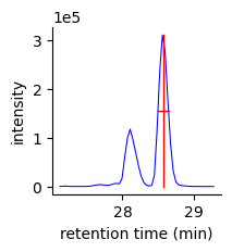
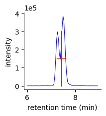
    # 2.
    xic_rt, xic_i = mza.collect_xic_arrays_by_mz(ref_mz - 0.01, ref_mz + 0.01,
                                                 rt_bounds=(exp_rt - 1.5, exp_rt + 1.5))
    pk_means, pk_heights, pk_widths = find_peaks_1d_gauss(xic_rt, xic_i,
                                                          0.05, 1e3, 0.05,
                                                          0.5, 1, True)
    obs_rt, obs_rt_fwhm = pk_means[0], pk_widths[0]
    print('obs. RT: {:.2f} +/- {:.2f} min'.format(obs_rt, obs_rt_fwhm))
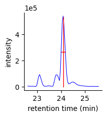
    print('XIC with fit:')
    ax = plot_chrom(xic_rt, xic_i,  figsize=(2., 2.))
    add_peaks_to_plot(ax, pk_means, pk_heights, pk_widths)
    plt.show()
    plt.close()
    # 3.
    atd_dt, atd_i = mza.collect_atd_arrays_by_rt_mz(ref_mz - 0.01, ref_mz + 0.01,
                                                    obs_rt - obs_rt_fwhm, obs_rt + obs_rt_fwhm)
    atd_means, atd_heights, atd_widths = find_peaks_1d_gauss(atd_dt, atd_i,
                                                             0.05, 1e3, 1,
                                                             20, 1, True)
    obs_dt, obs_dt_fwhm = atd_means[0], atd_widths[0]
    print('obs. DT: {:.2f} +/- {:.2f} ms'.format(obs_dt, obs_dt_fwhm))
    print('ATD with fit:')
    ax = plot_atd(atd_dt, atd_i,
                  dt_range=[obs_dt - 5, obs_dt + 5], figsize=(2., 2.))
    add_peaks_to_plot(ax, atd_means, atd_heights, atd_widths)
    plt.show()
    plt.close()
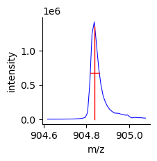
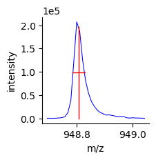
    # 4.
    ms1_mz, ms1_i = mza.collect_ms1_arrays_by_rt_dt(obs_rt - obs_rt_fwhm, obs_rt + obs_rt_fwhm,
                                                    obs_dt - obs_dt_fwhm, obs_dt + obs_dt_fwhm,
                                                    mz_bounds=[ref_mz - 0.25, ref_mz + 0.25])
    ms1_means, ms1_heights, ms1_widths = find_peaks_1d_gauss(ms1_mz, ms1_i,
                                                             0.05, 1e3, 0.015,
                                                             0.15, 1, True)
    obs_mz = ms1_means[0]
    print('obs. m/z: {:.6f}'.format(obs_mz))
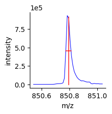
    print('MS1 with fit:')
    ax = plot_spectrum(ms1_mz, ms1_i, figsize=(2., 2.))
    add_peaks_to_plot(ax, ms1_means, ms1_heights, ms1_widths)
    plt.show()
    plt.close()
    # 5.
    return ref_mz, obs_mz

# Fetch observed m/z values for all of the mass calibrants

ref_mzs, obs_mzs = [], []
for calibrant in mass_calibrants:
    print('-' * 40)
    ref_mz, obs_mz = get_obs_mz(*calibrant)
    ref_mzs.append(ref_mz)
    obs_mzs.append(obs_mz)
print('-' * 40)

# convert to numpy ndarrays
ref_mzs, obs_mzs = np.array([ref_mzs, obs_mzs])

----------------------------------------
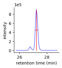
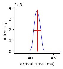
TG(50:1) [M+NH4]+
reference m/z: 850.786365
obs. RT: 27.69 +/- 0.17 min
XIC with fit:

obs. DT: 41.26 +/- 1.40 ms
ATD with fit:

obs. m/z: 850.791254
MS1 with fit:

----------------------------------------
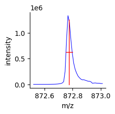
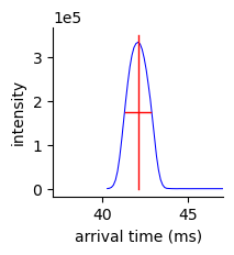
TG(52:4) [M+NH4]+
reference m/z: 872.770715
obs. RT: 24.09 +/- 0.18 min
XIC with fit:

obs. DT: 41.56 +/- 1.12 ms
ATD with fit:

obs. m/z: 872.774762
MS1 with fit:

----------------------------------------
TG(52:3) [M+NH4]+
reference m/z: 874.786365
obs. RT: 27.25 +/- 0.20 min
XIC with fit:

obs. DT: 41.51 +/- 1.47 ms
ATD with fit:

obs. m/z: 874.794993
MS1 with fit:

----------------------------------------
TG(52:1) [M+NH4]+
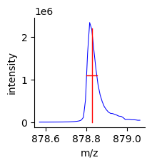
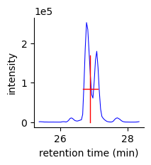
reference m/z: 878.817666
obs. RT: 28.15 +/- 0.18 min
XIC with fit:

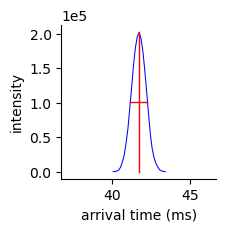
obs. DT: 42.09 +/- 1.49 ms
ATD with fit:

obs. m/z: 878.826442
MS1 with fit:

----------------------------------------
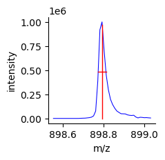
TG(54:5) [M+NH4]+
reference m/z: 898.786365
obs. RT: 26.89 +/- 0.44 min
XIC with fit:

obs. DT: 41.71 +/- 1.09 ms
ATD with fit:

obs. m/z: 898.791653
MS1 with fit:

----------------------------------------
TG(54:2) [M+NH4]+
reference m/z: 904.833316
obs. RT: 28.13 +/- 0.18 min
XIC with fit:

obs. DT: 42.61 +/- 1.31 ms
ATD with fit:

obs. m/z: 904.839460
MS1 with fit:

----------------------------------------
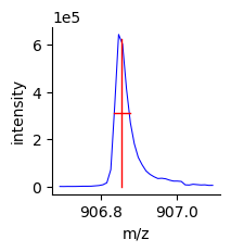
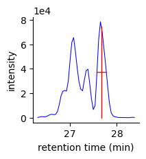
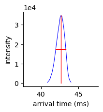
TG(54:1) [M+NH4]+
reference m/z: 906.848966
obs. RT: 28.57 +/- 0.15 min
XIC with fit:

obs. DT: 42.71 +/- 1.02 ms
ATD with fit:

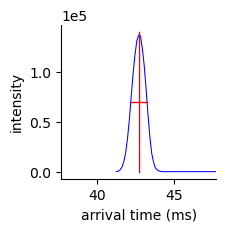
obs. m/z: 906.854695
MS1 with fit:

----------------------------------------
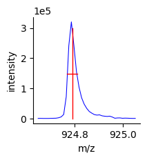
TG(56:6) [M+NH4]+
reference m/z: 924.802015
obs. RT: 27.67 +/- 0.20 min
XIC with fit:

obs. DT: 42.65 +/- 1.31 ms
ATD with fit:

obs. m/z: 924.791458
MS1 with fit:

----------------------------------------
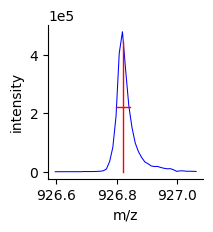
TG(56:5) [M+NH4]+
reference m/z: 926.817666
obs. RT: 27.47 +/- 0.37 min
XIC with fit:

obs. DT: 42.72 +/- 1.05 ms
ATD with fit:

obs. m/z: 926.820352
MS1 with fit:

----------------------------------------
TG(58:8) [M+NH4]+
reference m/z: 948.802015
obs. RT: 27.00 +/- 0.16 min
XIC with fit:

obs. DT: 42.80 +/- 1.00 ms
ATD with fit:

obs. m/z: 948.806533
MS1 with fit:

----------------------------------------

# construct the calibration
mz_cal = MassCalibration(ref_mzs, obs_mzs, 'linear')

# plot calibration results
plot_mass_calibration(mz_cal, figname='show')

CCS Calibration

# use some lipids from this sample as mass calibrants
# lipid id, molecular formula (neutral), ionization, expected retention time, ref. CCS
ccs_calibrants = [
    ['PE(18:1_0:0)', MolecularFormula(C=23, H=46, O=7, N=1, P=1), '[M+H]+', 7.491, 215.8],
    ['PC(18:1_0:0)', MolecularFormula(C=26, H=52, O=7, N=1, P=1), '[M+H]+', 7.301, 235.6],
    ['PE(18:1/18:1)', MolecularFormula(C=41, H=78, O=8, N=1, P=1), '[M+H]+', 19.869, 280.6],
    ['PC(18:1/18:1)', MolecularFormula(C=44, H=84, O=8, N=1, P=1), '[M+H]+', 19.793, 297.3],
    ['TG(52:1)', MolecularFormula(C=55, H=104, O=6), '[M+NH4]+', 28.165, 323.6],
]

# define a function for extracting the observed arrival times and ref. m/z values
# for calibrants from the data file
def get_mz_dt(lipid, neutral_formula, adduct, exp_rt, ref_ccs):
    """
    1. Using the lipid molecular formula and adduct, compute reference accurate m/z
    2. Extract XIC from near the expected RT, fit to obtain observed RT and peak width
    3. Extract an RT-filtered ATD, fit to obtain observed arrival time and peak width
    4. Return reference m/z and observed arrival time values (+ pass through ref ccs)
    """
    # 1.
    print(lipid, adduct)
    ref_mz = ms_adduct_mz(neutral_formula, adduct)
    print('reference m/z: {:.6f}'.format(ref_mz))
    # 2.
    xic_rt, xic_i = mza.collect_xic_arrays_by_mz(ref_mz - 0.01, ref_mz + 0.01,
                                                 rt_bounds=(exp_rt - 1.5, exp_rt + 1.5))
    pk_means, pk_heights, pk_widths = find_peaks_1d_gauss(xic_rt, xic_i,
                                                          0.05, 1e3, 0.05,
                                                          0.5, 1, True)
    obs_rt, obs_rt_fwhm = pk_means[0], pk_widths[0]
    print('obs. RT: {:.2f} +/- {:.2f} min'.format(obs_rt, obs_rt_fwhm))
    print('XIC with fit:')
    ax = plot_chrom(xic_rt, xic_i,  figsize=(2., 2.))
    add_peaks_to_plot(ax, pk_means, pk_heights, pk_widths)
    plt.show()
    plt.close()
    # 3.
    atd_dt, atd_i = mza.collect_atd_arrays_by_rt_mz(ref_mz - 0.01, ref_mz + 0.01,
                                                    obs_rt - obs_rt_fwhm, obs_rt + obs_rt_fwhm)
    atd_means, atd_heights, atd_widths = find_peaks_1d_gauss(atd_dt, atd_i,
                                                             0.05, 1e3, 1,
                                                             20, 1, True)
    obs_dt, obs_dt_fwhm = atd_means[0], atd_widths[0]
    print('obs. DT: {:.2f} +/- {:.2f} ms'.format(obs_dt, obs_dt_fwhm))
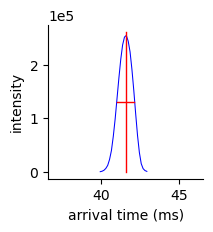
    print('ATD with fit:')
    ax = plot_atd(atd_dt, atd_i,
                  dt_range=[obs_dt - 5, obs_dt + 5], figsize=(2., 2.))
    add_peaks_to_plot(ax, atd_means, atd_heights, atd_widths)
    plt.show()
    plt.close()
    # 4.
    return ref_mz, obs_dt, ref_ccs

# Fetch observed arrival time values for all of the CCS calibrants

ref_mzs, obs_dts, ref_ccss = [], [], []
for calibrant in ccs_calibrants:
    print('-' * 40)
    ref_mz, obs_dt, ref_ccs = get_mz_dt(*calibrant)
    ref_mzs.append(ref_mz)
    obs_dts.append(obs_dt)
    ref_ccss.append(ref_ccs)
print('-' * 40)

# convert to numpy ndarrays
ref_mzs, obs_dts, ref_ccss = np.array([ref_mzs, obs_dts, ref_ccss])

----------------------------------------
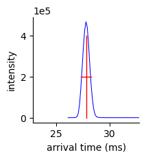
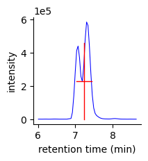
PE(18:1_0:0) [M+H]+
reference m/z: 480.309015
obs. RT: 7.42 +/- 0.39 min
XIC with fit:

obs. DT: 27.79 +/- 1.00 ms
ATD with fit:

----------------------------------------
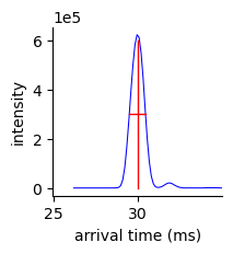
PC(18:1_0:0) [M+H]+
reference m/z: 522.355965
obs. RT: 7.23 +/- 0.42 min
XIC with fit:

obs. DT: 29.97 +/- 1.00 ms
ATD with fit:

----------------------------------------
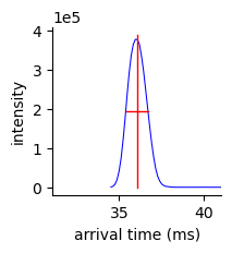
PE(18:1/18:1) [M+H]+
reference m/z: 744.554331
obs. RT: 19.90 +/- 0.36 min
XIC with fit:

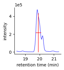
obs. DT: 36.05 +/- 1.28 ms
ATD with fit:

----------------------------------------
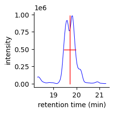
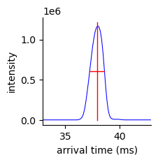
PC(18:1/18:1) [M+H]+
reference m/z: 786.601281
obs. RT: 19.71 +/- 0.50 min
XIC with fit:

obs. DT: 37.93 +/- 1.30 ms
ATD with fit:

----------------------------------------
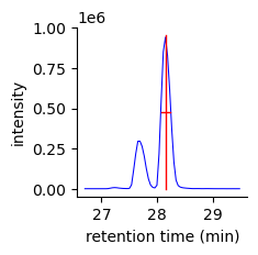
TG(52:1) [M+NH4]+
reference m/z: 878.817666
obs. RT: 28.15 +/- 0.18 min
XIC with fit:

obs. DT: 42.09 +/- 1.49 ms
ATD with fit:

----------------------------------------

# construct the calibration (z=1)
ccs_cal = CCSCalibrationDTsf(ref_mzs, obs_dts, ref_ccss, 1)

# plot calibration results
plot_dtsf_ccs_calibration(ccs_cal, figname='show')

Cleanup

# close the MZA interface
mza.close()